Twenty-Five Things You Didn’t Know You Could Do with R

Twenty-Five Things You Didn’t Know You Could Do with R

Hi, I’m David Keyes and I run R for the Rest of Us. I’m excited to be here today and to talk with you about doing things in R you didn’t know you could do. Twenty-five things to be precise.

I find it ironic in many ways that I am up here talking to you about unique ways to use R. I say that because for a long time I didn’t feel like a “real” R user. You see, I don’t come from a typical R background. I’m a qualitative researcher with a PhD in anthropology. I don’t have advanced training in statistics. When I started using R I felt like I wasn’t a real R user because the most complicated stats I calculated then, and still calculate now, were descriptive stats.

But eventually I realized that R isn’t just about stats. Or, more precisely, R can do more than just complicated statistical techniques. Eventually, I learned to use R for things like data visualization, reproducible reporting, making maps, and much more. R became my Swiss Army knife, enabling me to do anything I needed to with data.

And the more I started talking with others about how I used R, they were, to my surprise, quite interested. Eventually, I came to peace with how I used R. I didn’t need to do complicated statistics to be a real R user. And, in fact, even among people who do use R for complicated stats, R’s capabilities as a more general purpose tool are extremely appealing. My goal today is to show you a few things that you can do with R that you may never have considered.

Now, before I get started, just one thing: not everything you will hear me talk about today is going to be new to you. It’s impossible to choose twenty-five things that no one in a group of this size will be familiar with. But my hope is that you come away with at least a few new ideas for ways you can use R that you never previously considered.

1. Access Data Automagically
2. Efficiently Make Beautiful Data Viz
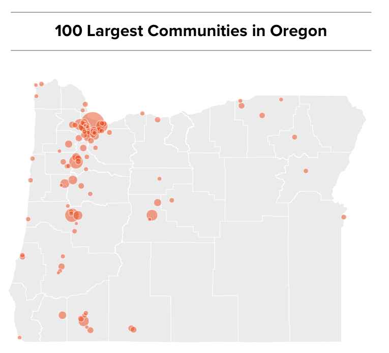
3. Make Maps
4. Report in New Ways with Quarto
5. Automate all the Things
6. Use AI to Write Better Code
7. Use AI to Analyze Data

https://rfortherestofus.com/cascadia2025

Access Data Automagically

Before you do any work in R, you need data. Let’s begin by talking about ways that you can access data directly from R.

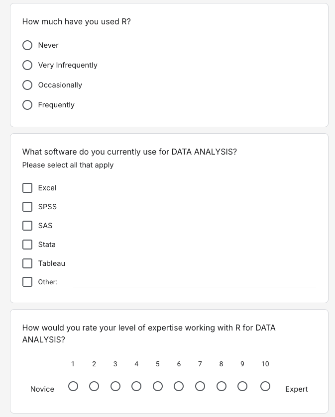
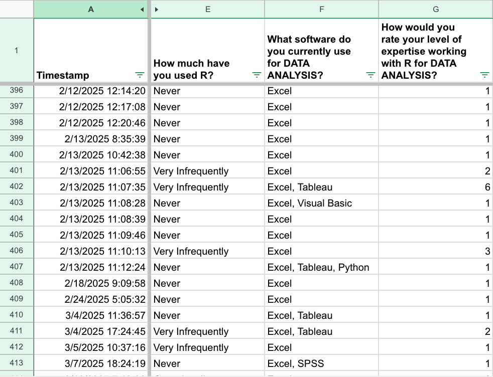
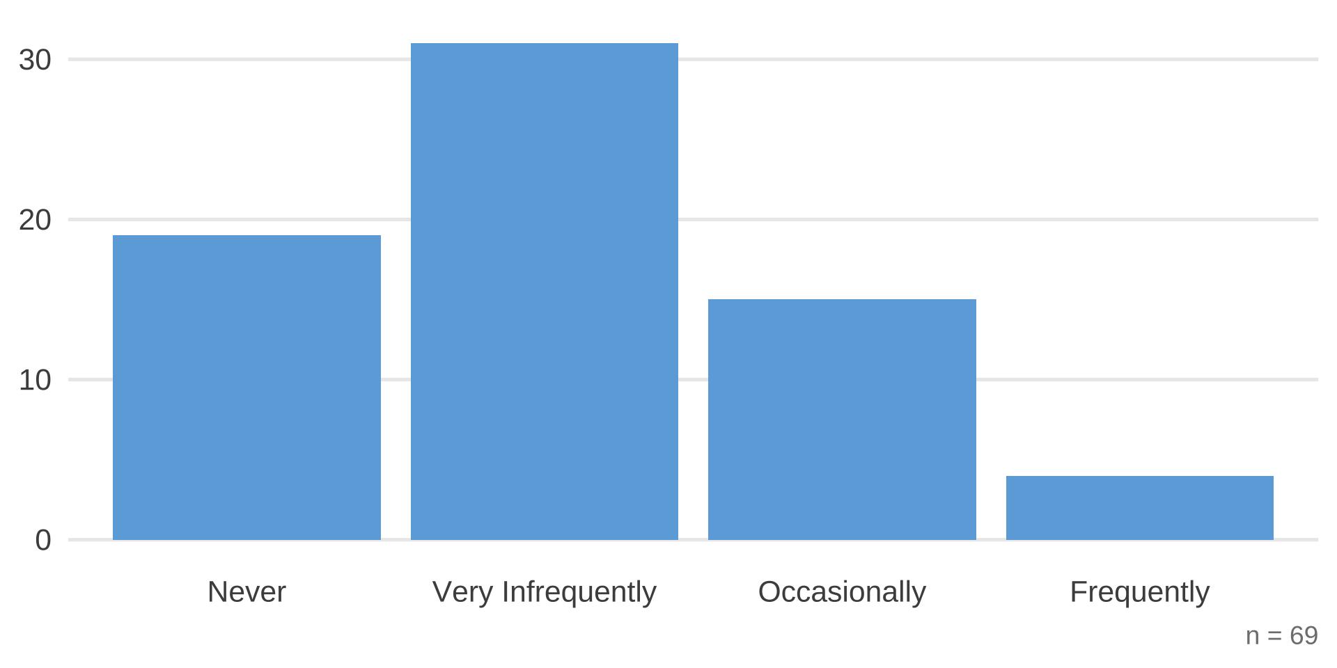
Pull in Data Directly from Google Sheets

1

As a social scientist, I conduct a lot of surveys. Now that I use R, one of my favorite ways to conduct surveys is with Google Forms.

Using Google Forms allows me to put survey responses directly into Google Sheets.

library(googlesheets4)

survey_data <-
  read_sheet(sheet = "YOURSHEETURLHERE")

And having data in Google Sheets allows me to use the {googlesheets4} package to access that data directly from R.

Spring 2024

Fall 2024

This means that every time a new response comes in, it just takes you rerunning your code in order to create new analysis, data viz, etc.

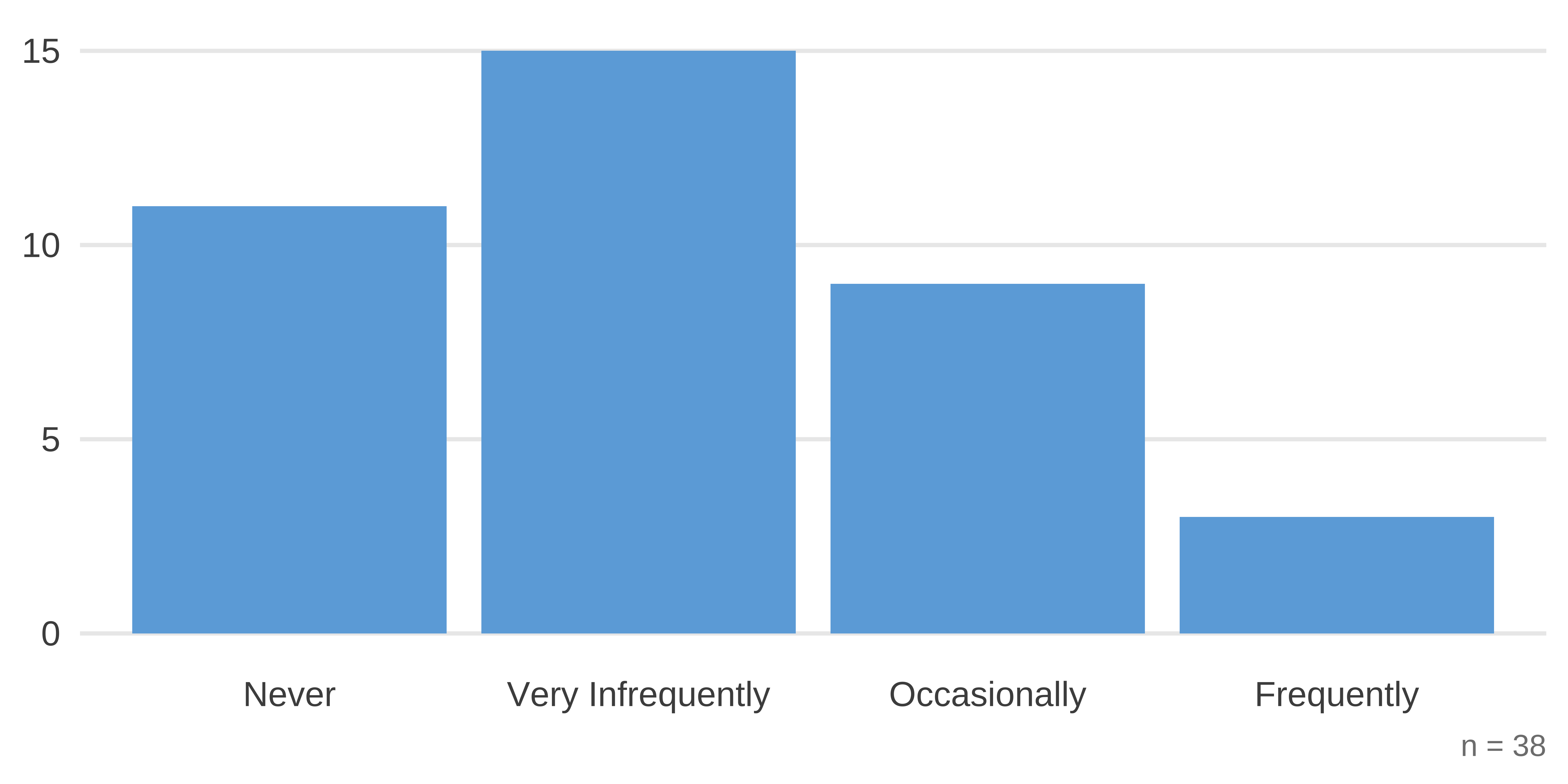
Pull in Data Directly from Qualtrics

2

library(qualtRics)

survey_data <-
  fetch_survey(surveyID = "YOURSURVEYIDHERE")

Another common tool for those collecting surveys is Qualtrics. And, fortunately for you, if you use Qualtrics, there is a package to bring in data directly from it. With the fetch_survey() function, you can bring in data from a Qualtrics survey, ensuring you are always working with the most up-to-date data.

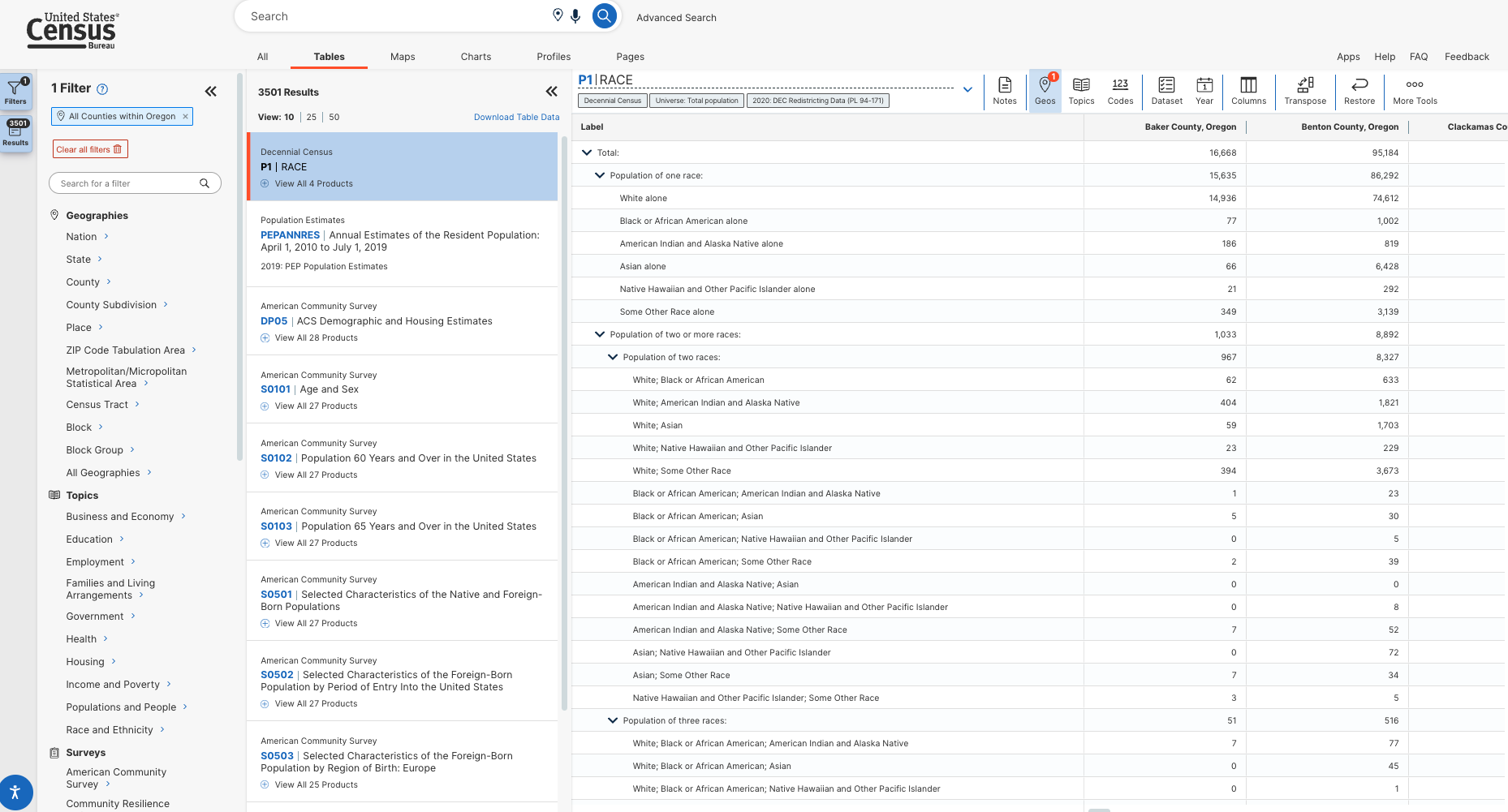
Pull in Data Directly from the Census Bureau

3

Before I used R, I would spend hours on the Census Bureau website, finding the data I needed, downloading it, and then working with it in Excel.

A third way that I like to connect directly to my data source is with the {tidycensus} package. I work with a lot of data from the Census Bureau.

library(tidycensus)

get_acs(
  state = "OR",
  geography = "place",
  geometry = TRUE,
  variables = "B01003_001"
)

But with the {tidycensus} package, I can connect directly to the Census Bureau, pulling in data on command.

This approach has proven particularly helpful in my work on the annual Oregon by the Numbers report, which relies heavily on data from the American Community Survey.

Simple feature collection with 426 features and 5 fields
Geometry type: MULTIPOLYGON
Dimension:     XY
Bounding box:  xmin: -124.5125 ymin: 41.99277 xmax: -116.9354 ymax: 46.20566
Geodetic CRS:  NAD83
First 10 features:
     GEOID                      NAME   variable estimate moe
1  4149600       Monroe city, Oregon B01003_001      853 272
2  4181300      Wheeler city, Oregon B01003_001      429 137
3  4150050       Mosier city, Oregon B01003_001      630 262
4  4176250        Unity city, Oregon B01003_001       37  20
5  4133250        Helix city, Oregon B01003_001      358 185
6  4149150     Mitchell city, Oregon B01003_001      202 107
7  4161700     Richland city, Oregon B01003_001      199  74
8  4129950    Gold Hill city, Oregon B01003_001     1261 270
9  4153150 North Plains city, Oregon B01003_001     3365  43
10 4104000       Barlow city, Oregon B01003_001      157 105
                         geometry
1  MULTIPOLYGON (((-123.3067 4...
2  MULTIPOLYGON (((-123.9055 4...
3  MULTIPOLYGON (((-121.4047 4...
4  MULTIPOLYGON (((-118.1944 4...
5  MULTIPOLYGON (((-118.6616 4...
6  MULTIPOLYGON (((-120.1641 4...
7  MULTIPOLYGON (((-117.1722 4...
8  MULTIPOLYGON (((-123.0729 4...
9  MULTIPOLYGON (((-123.0114 4...
10 MULTIPOLYGON (((-122.7278 4...

Work with APIs to Access Data

4

Under the hood, the {googlesheets4}, {qualtRics}, and {tidycensus} packages connect to data sources through APIs. Fortunately for us, they hide the often complicated work of accessing data through APIs. Unfortunately for us, there are times when we need to access data available through APIs, but without a wrapper package to simplify the process. In this case, the {httr2} package enables us to connect directly with APIs.

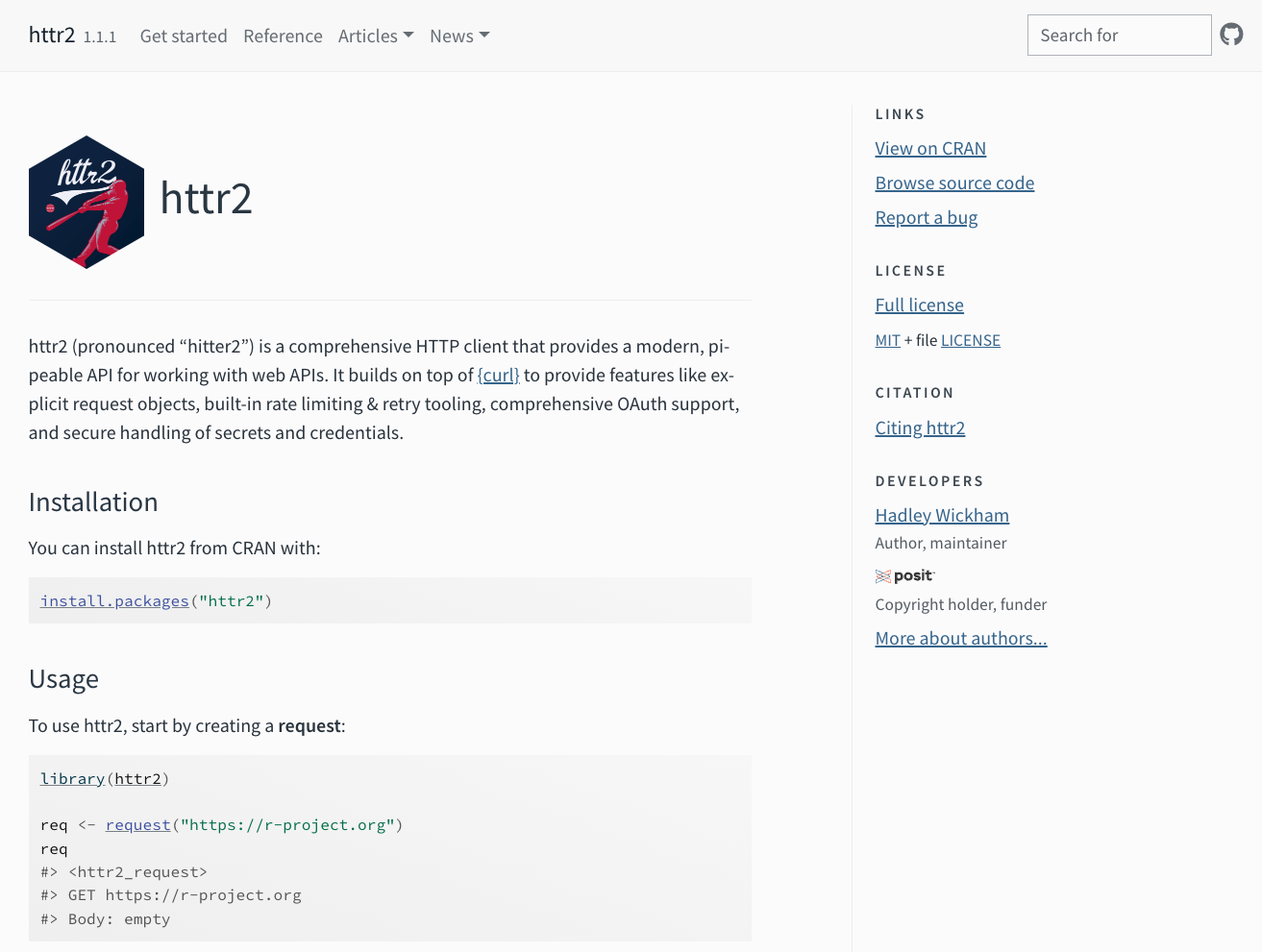
library(httr2)

fathom_api_key <- Sys.getenv("FATHOM_API_KEY")

request("https://api.usefathom.com/v1/aggregations") |>
  req_url_query(
    entity = "pageview",
    aggregates = "visits,uniques,pageviews",
    sort_by = "visits:desc"
  ) |>
  req_headers(
    Authorization = str_glue("Bearer {fathom_api_key}")
  ) |>
  req_perform()

Since few of these tools have dedicated R packages, I write code to connect to them directly.

# A tibble: 28,976 × 5
   url                                       date       visits uniques pageviews
   <glue>                                    <date>      <dbl>   <dbl>     <dbl>
 1 /2018/06/the-life-changing-magic-of-r/    2021-03-01      4       9         9
 2 /2018/07/r-handles-the-beast-and-the-bea… 2021-03-01      1       3         3
 3 /2018/09/making-small-multiples-in-r/     2021-03-01     45      72        99
 4 /2018/12/descriptive-stats-r/             2021-03-01     11      47        52
 5 /2019/01/reproducibility-for-the-rest-of… 2021-03-01      1      36        41
 6 /2019/03/my-r-journey-dana-wanzer/        2021-03-01      2      12        12
 7 /2019/03/r-killer-feature-rmarkdown/      2021-03-01     37     216       258
 8 /2019/04/curb-cuts-universal-design-welc… 2021-03-01      8      18        20
 9 /2019/04/my-r-journey-david-keyes/        2021-03-01     23      78        94
10 /2019/04/my-r-journey-rika-gorn/          2021-03-01      0       3         3
# ℹ 28,966 more rows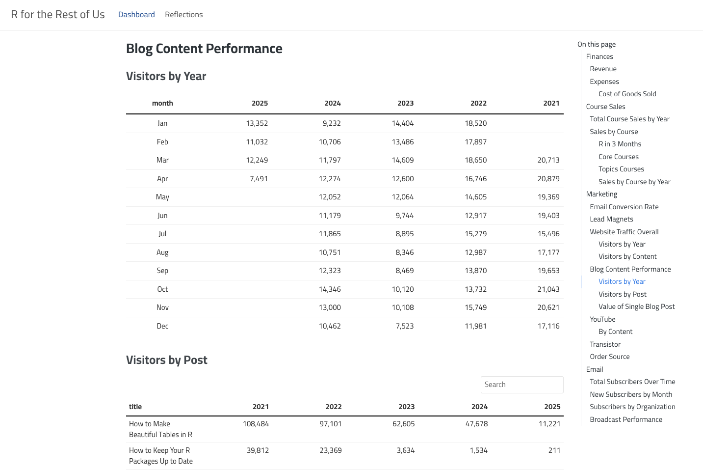

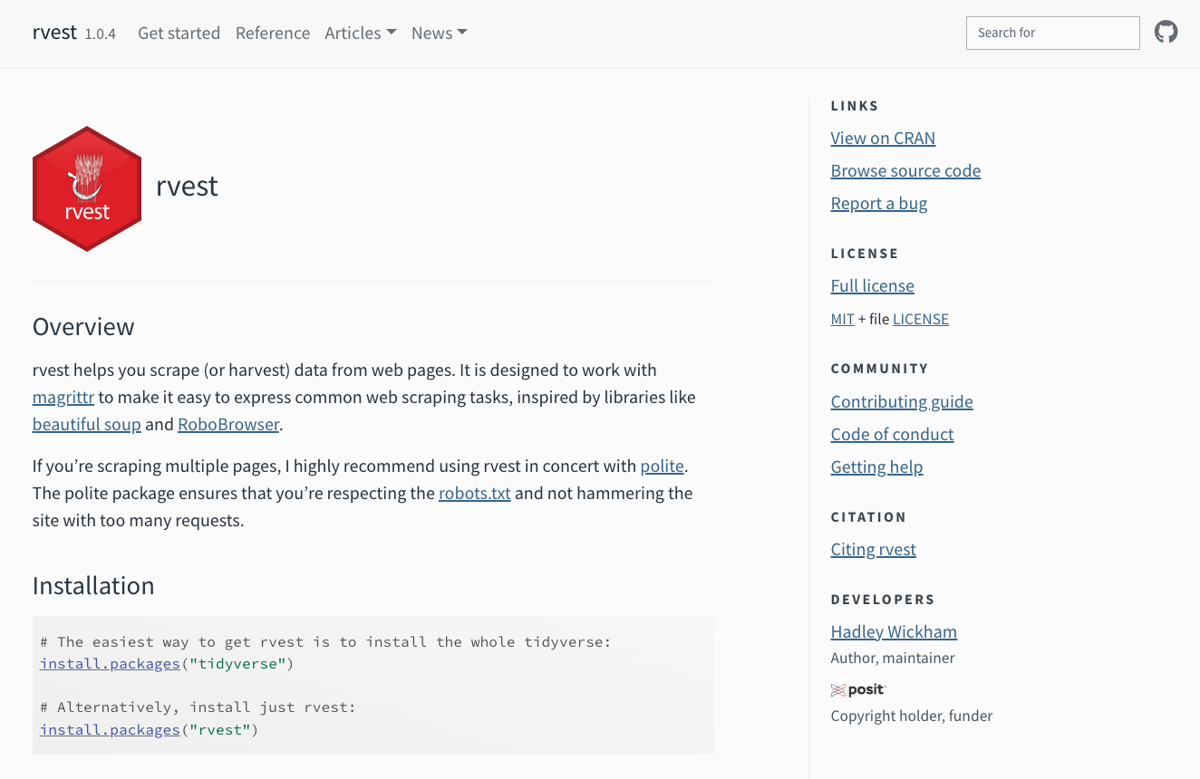
For example, I have an internal dashboard I use to pull in data from multiple sources.

Scrape Data

5

There are other times when we want to access data and is there is no package to access it, nor is there an API to enable us to connect to the data source. In this case, we often need to scrape data from webpages. The {rvest} package is your friend in this case.

library(rvest)
library(tidyverse)

read_html("https://en.wikipedia.org/wiki/List_of_FIFA_World_Cup_finals") |>
  html_elements("table") |>
  pluck(4) |>
  html_table() |>
  select(-Ref.)

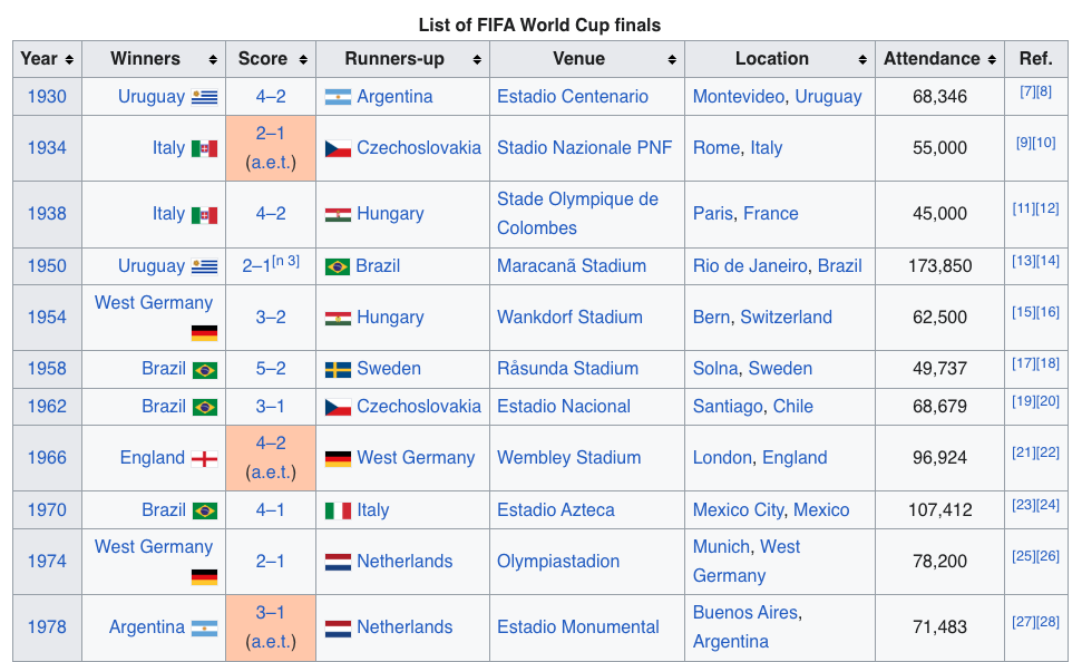
# A tibble: 23 × 7
    Year Winners      Score        `Runners-up`   Venue      Location Attendance
   <int> <chr>        <chr>        <chr>          <chr>      <chr>    <chr>     
 1  1930 Uruguay      4–2          Argentina      Estadio C… Montevi… 68,346    
 2  1934 Italy        2–1 (a.e.t.) Czechoslovakia Stadio Na… Rome, I… 55,000    
 3  1938 Italy        4–2          Hungary        Stade Oly… Paris, … 45,000    
 4  1950 Uruguay      2–1[n 3]     Brazil         Maracanã … Rio de … 173,850   
 5  1954 West Germany 3–2          Hungary        Wankdorf … Bern, S… 62,500    
 6  1958 Brazil       5–2          Sweden         Råsunda S… Solna, … 49,737    
 7  1962 Brazil       3–1          Czechoslovakia Estadio N… Santiag… 68,679    
 8  1966 England      4–2 (a.e.t.) West Germany   Wembley S… London,… 96,924    
 9  1970 Brazil       4–1          Italy          Estadio A… Mexico … 107,412   
10  1974 West Germany 2–1          Netherlands    Olympiast… Munich,… 78,200    
# ℹ 13 more rows

Efficiently Make Beautiful Data Viz

Make Your Own ggplot Theme

6

If you make plots in ggplot (and if you’re here, I’m guessing you do), keeping them consistent and on brand can be challenging. Fortunately, this is where themes come in. If you’ve never tried to make your own ggplot theme, you should! It’s surprisingly simple and with a few lines of code you can ensure that all of your plots are on brand.

penguins_bar_chart

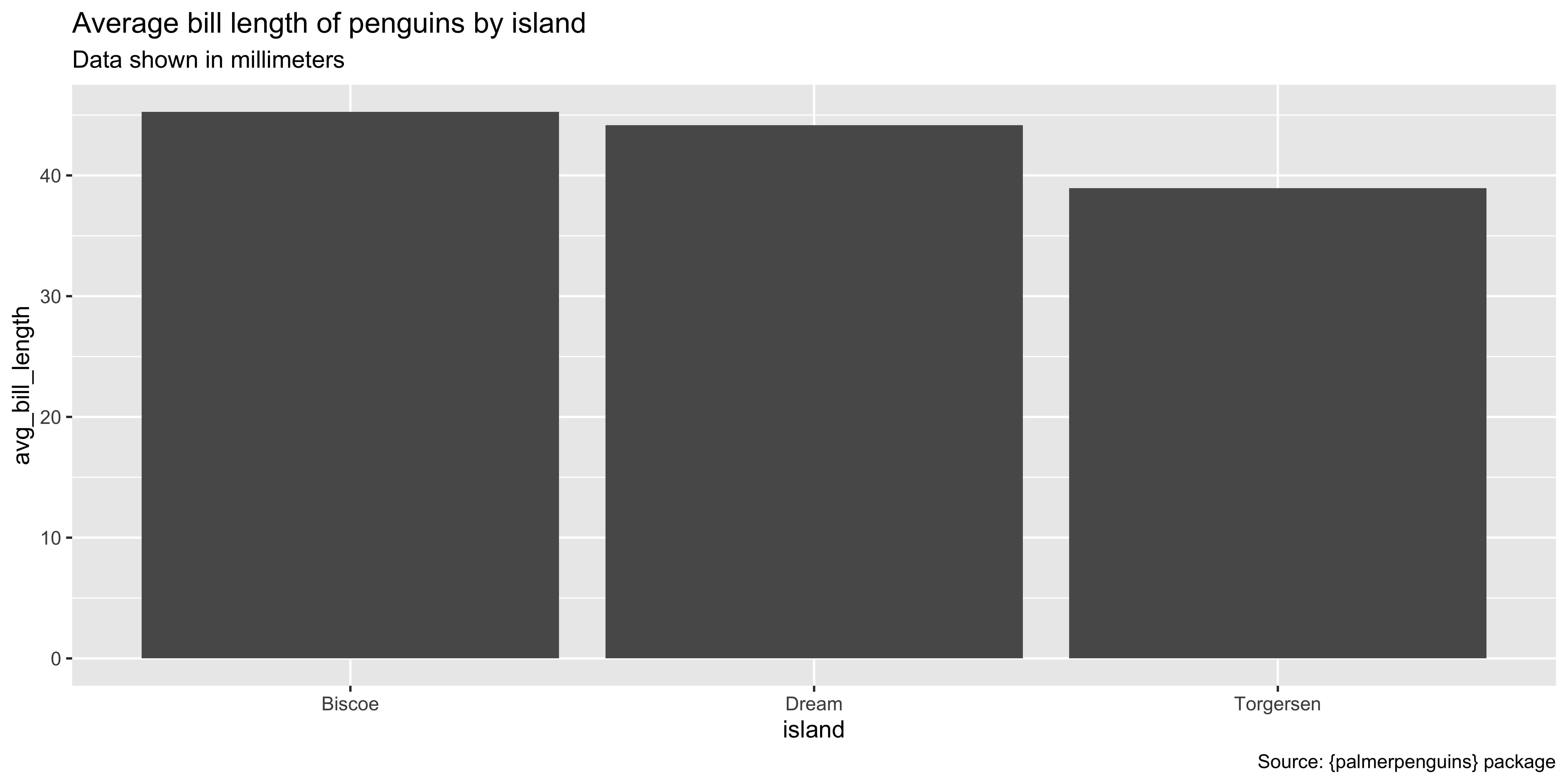
library(tidyverse)

theme_dk <- function(base_family = "Inter Tight", base_size = 14) {
  theme_minimal(base_size = base_size, base_family = base_family) +
    theme(
      panel.grid.minor = element_blank(),
      panel.grid.major = element_line(
        color = "grey90",
        linewidth = 0.5,
        linetype = "dashed"
      ),
      axis.text = element_text(
        color = "grey50"
      ),
      ETC
    )
}

penguins_bar_chart +
  theme_dk()

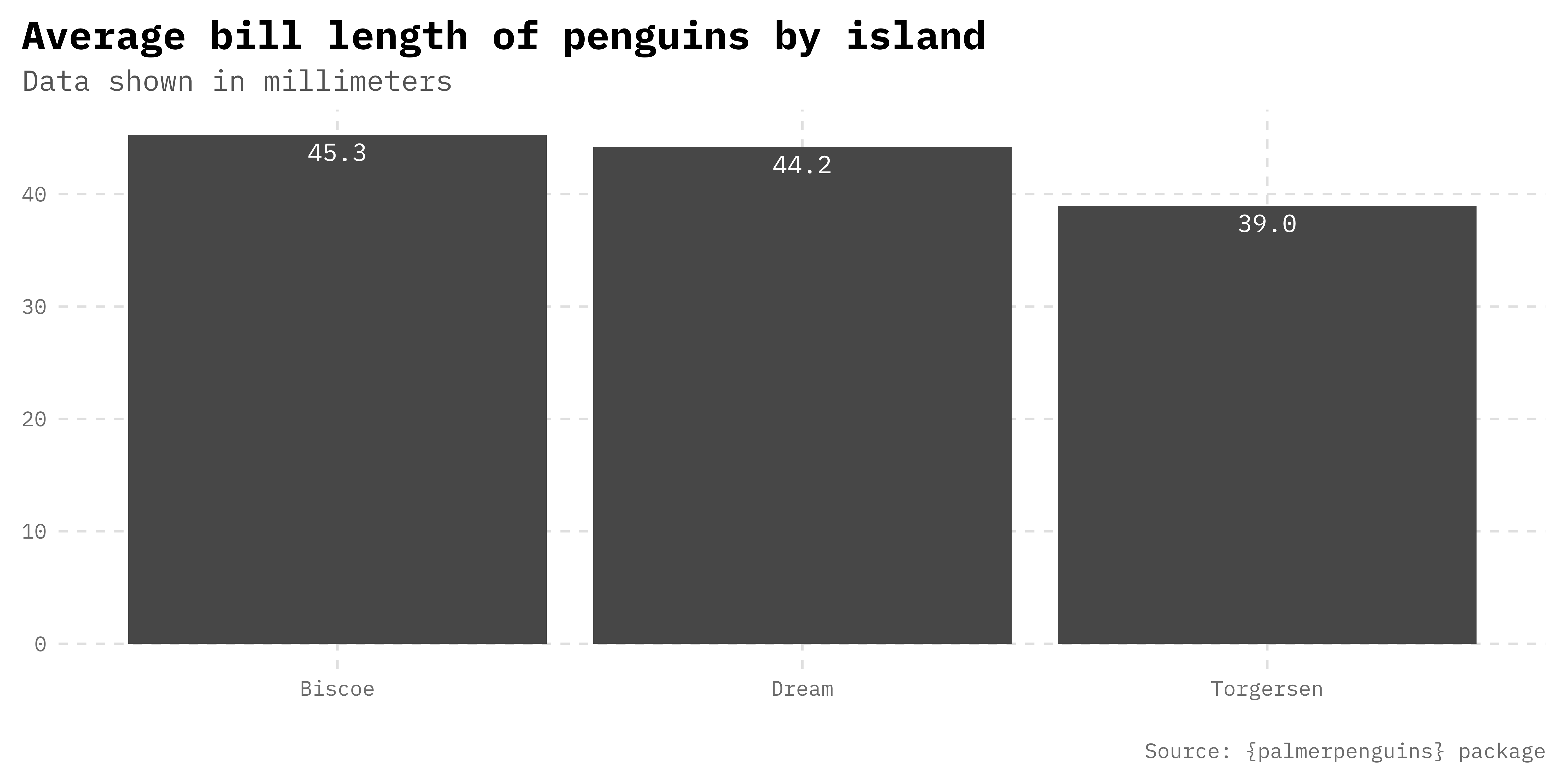
Use Your Theme Everywhere

7

theme_set(theme_dk())

---
title: "Penguins Report"
---

```{r}
theme_dk <- function(base_family = "Inter Tight", base_size = 14) {}
```

```{r}
theme_set(theme_dk())
```

```{r}
penguins_bar_chart
```

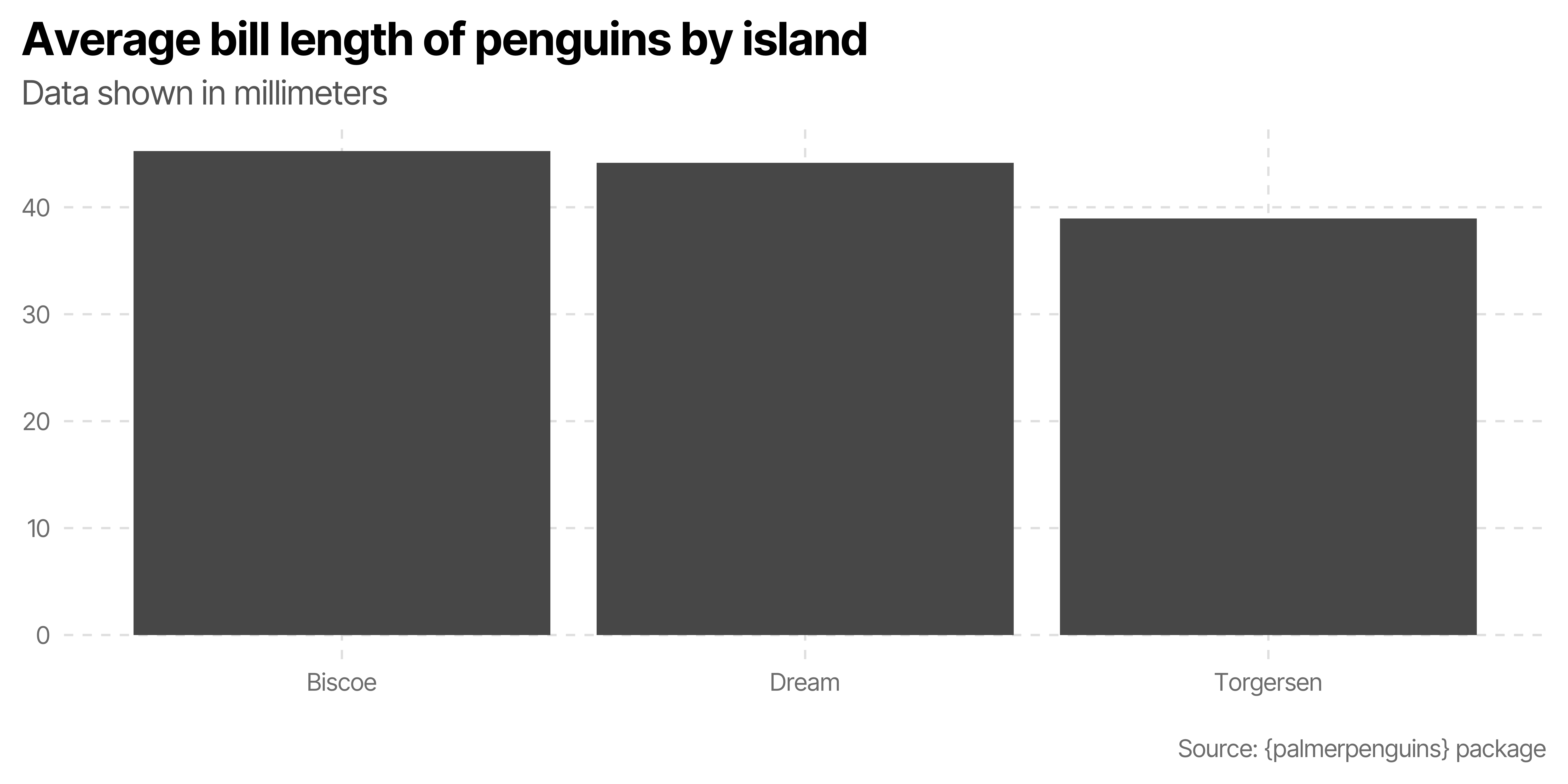
Make Your Text Consistent with Your Theme

8

Creating a theme is a great way to handle the look and feel of things like titles, axis text, grid lines, etc. What themes do not change is text added through geoms.

penguins_bar_chart +
  theme_dk(base_family = "IBM Plex Mono", base_size = 12) +
  geom_text(
    aes(label = avg_bill_length_formatted),
    vjust = 1.5,
    color = "white",
    size = 4
  )

So, let’s say you want to use geom_text() to add labels to your plot. See here how I’ve added a layer to my plot to add labels that show the average bill length. You’ll also see that I’ve changed the font in my theme to be IBM Plex Mono just to make it more obvious.

When I run my code I get a plot that uses IBM Plex Mono everywhere except where geom_text() added labels.

penguins_bar_chart +
  theme_dk(base_family = "IBM Plex Mono", base_size = 12) +
  geom_text(
    aes(label = avg_bill_length_formatted),
    vjust = 1.5,
    color = "white",
    family = "IBM Plex Mono",
    size = 4
  )

The way most people change this is by adding family = "IBM Plex Mono" within geom_text(). This is fine to do in one or two charts, but say you’re making an entire report with dozens of charts. You don’t want to have to add family = "IBM Plex Mono" dozens of times. The way around this is with the update_geom_defaults() function. This function lets you set defaults for various geoms.

update_geom_defaults(
  geom = "text",
  aes(family = "IBM Plex Mono")
)

Here, for example, you can set the default family for all geom_text() instances to be IBM Plex Mono.

---
title: "Penguins Report"
---

```{r}
theme_dk <- function()
```

```{r}
theme_set(theme_dk())

update_geom_defaults(geom = "text", aes(family = "IBM Plex Mono"))
```

```{r}
penguins_bar_chart +
  geom_text(
    aes(label = avg_bill_length_formatted),
    vjust = 1.5,
    color = "white",
    size = 4
  )
```

Just put this code at the top of your R script or Quarto document and all of your charts will use IBM Plex Mono everywhere.

Make Maps

Make Maps with ggplot

9

R is renowned for its graph-making capabilities. Did you know that you can use ggplot, that same package you use to make graphs, to make maps? There is a special geom (geom_sf()) that allows you to make maps. And everything you have learned about ggplot applies to maps too: color and fill scales, themes, and more.

library(tidycensus)

median_income_by_county <-
  get_acs(
    geography = "county",
    variables = c(median_income = "B19013_001"),
    geometry = TRUE
  )

median_income_by_county

Simple feature collection with 3222 features and 5 fields
Geometry type: MULTIPOLYGON
Dimension:     XY
Bounding box:  xmin: -179.1467 ymin: 17.88328 xmax: 179.7785 ymax: 71.38782
Geodetic CRS:  NAD83
First 10 features:
   GEOID                           NAME      variable estimate   moe
1  01069        Houston County, Alabama median_income    55064  1412
2  01023        Choctaw County, Alabama median_income    43299  8544
3  01005        Barbour County, Alabama median_income    39712  3289
4  01107        Pickens County, Alabama median_income    45339  2865
5  01033        Colbert County, Alabama median_income    56149  3200
6  04012         La Paz County, Arizona median_income    46634  2584
7  04001         Apache County, Arizona median_income    37483  3091
8  05081  Little River County, Arkansas median_income    58627 11485
9  05121      Randolph County, Arkansas median_income    45993  4649
10 06037 Los Angeles County, California median_income    83411   439
                         geometry
1  MULTIPOLYGON (((-85.71209 3...
2  MULTIPOLYGON (((-88.47323 3...
3  MULTIPOLYGON (((-85.74803 3...
4  MULTIPOLYGON (((-88.34043 3...
5  MULTIPOLYGON (((-88.13925 3...
6  MULTIPOLYGON (((-114.7312 3...
7  MULTIPOLYGON (((-110.0007 3...
8  MULTIPOLYGON (((-94.48558 3...
9  MULTIPOLYGON (((-91.40687 3...
10 MULTIPOLYGON (((-118.6044 3...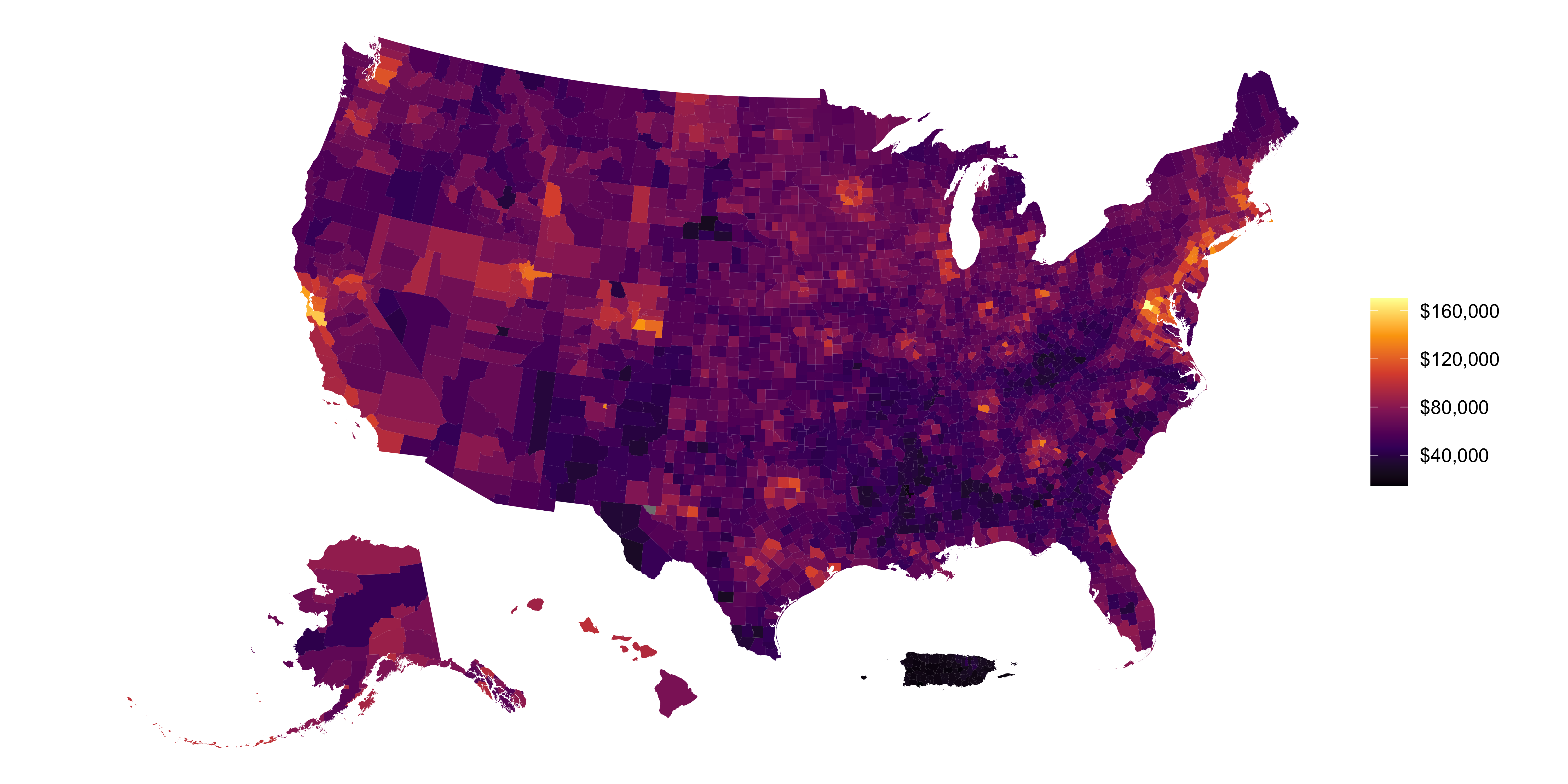

library(tidyverse)
library(tigris)
library(scales)

median_income_by_county |>
  shift_geometry() |>
  ggplot(aes(fill = estimate)) +
  geom_sf(linewidth = 0) +
  scale_fill_viridis_c(
    option = "B",
    labels = dollar_format(),
    name = NULL
  ) +
  theme_void()

Do Geospatial Analysis

10

It’s not just mapping that you can do in R. If you need to do geospatial analysis in R, that’s very possible! While many people think of tools like ArcGIS for geospatial analysis, R is a fully-fledged GIS tool. A client we work with recently asked me to do an analysis of SNAP-Ed program sites within 5 miles of grocery stores. With just a few lines of code, I was able to tell her the sites that met this criteria. This is just one example of how you can use R for geospatial analysis.

Reference https://github.com/MichiganFitnessFoundation/mff-r-training/issues/74

Which Elementary Schools in Portland are Within One Mile of a Public Library?

library(sf)

portland_libraries <- read_sf("data/portland_libraries.geojson")

Simple feature collection with 21 features and 1 field
Geometry type: POINT
Dimension:     XY
Bounding box:  xmin: -122.835 ymin: 45.44795 xmax: -122.479 ymax: 45.59008
Geodetic CRS:  WGS 84
# A tibble: 21 × 2
   library                                  geometry
   <chr>                                 <POINT [°]>
 1 West Slope Community Library (-122.7573 45.49324)
 2 St. Johns Library            (-122.7512 45.59008)
 3 North Portland Library       (-122.6715 45.56252)
 4 Sellwood-Moreland Library     (-122.6528 45.4677)
 5 Gregory Heights Library      (-122.5814 45.55157)
 6 Rockwood Library              (-122.479 45.51949)
 7 Midland Library              (-122.5382 45.51677)
 8 Hollywood Library            (-122.6216 45.53763)
 9 Belmont Library              (-122.6227 45.51524)
10 Central Library               (-122.683 45.51922)
# ℹ 11 more rows

portland_libraries_one_mile_buffer <-
  portland_libraries |>
  st_buffer(1609.34)

Simple feature collection with 21 features and 1 field
Geometry type: POLYGON
Dimension:     XY
Bounding box:  xmin: -122.8561 ymin: 45.43334 xmax: -122.4579 ymax: 45.60477
Geodetic CRS:  WGS 84
# A tibble: 21 × 2
   library                                                              geometry
 * <chr>                                                           <POLYGON [°]>
 1 West Slope Community Library ((-122.7586 45.4787, -122.7584 45.47877, -122.7…
 2 St. Johns Library            ((-122.7652 45.60085, -122.7654 45.60078, -122.…
 3 North Portland Library       ((-122.6812 45.57536, -122.6813 45.57533, -122.…
 4 Sellwood-Moreland Library    ((-122.667 45.45705, -122.6669 45.45693, -122.6…
 5 Gregory Heights Library      ((-122.6022 45.55156, -122.6024 45.5515, -122.6…
 6 Rockwood Library             ((-122.4592 45.52356, -122.459 45.52363, -122.4…
 7 Midland Library              ((-122.5348 45.53109, -122.5349 45.53106, -122.…
 8 Hollywood Library            ((-122.6421 45.53946, -122.6424 45.53935, -122.…
 9 Belmont Library              ((-122.6021 45.51627, -122.6019 45.51633, -122.…
10 Central Library              ((-122.6833 45.53382, -122.6835 45.53375, -122.…
# ℹ 11 more rows

pps_elementary_schools <-
  read_sf("data/pps_elementary_schools.geojson")

Simple feature collection with 86 features and 1 field
Geometry type: POINT
Dimension:     XY
Bounding box:  xmin: -122.893 ymin: 45.44022 xmax: -122.4617 ymax: 45.65579
Geodetic CRS:  WGS 84
# A tibble: 86 × 2
   school                                           geometry
   <chr>                                         <POINT [°]>
 1 Lenox Elementary School               (-122.893 45.55811)
 2 Cedar Mill Elementary School         (-122.7827 45.52651)
 3 Montclair Elementary School          (-122.7559 45.47644)
 4 Raleigh Hills Elementary School      (-122.7587 45.48163)
 5 Raleigh Park Elementary School       (-122.7576 45.49301)
 6 Ridgewood Elementary School          (-122.7786 45.50341)
 7 Rock Creek Elementary School         (-122.8676 45.55109)
 8 Terra Linda Elementary School        (-122.8244 45.53416)
 9 West Tualatin View Elementary School (-122.7662 45.51553)
10 William Walker Elementary School     (-122.7982 45.50076)
# ℹ 76 more rows

pps_elementary_schools |>
  st_join(portland_libraries_one_mile_buffer)

Simple feature collection with 89 features and 2 fields
Geometry type: POINT
Dimension:     XY
Bounding box:  xmin: -122.893 ymin: 45.44022 xmax: -122.4617 ymax: 45.65579
Geodetic CRS:  WGS 84
# A tibble: 89 × 3
   school                                           geometry library            
 * <chr>                                         <POINT [°]> <chr>              
 1 Lenox Elementary School               (-122.893 45.55811) <NA>               
 2 Cedar Mill Elementary School         (-122.7827 45.52651) <NA>               
 3 Montclair Elementary School          (-122.7559 45.47644) Garden Home Commun…
 4 Raleigh Hills Elementary School      (-122.7587 45.48163) West Slope Communi…
 5 Raleigh Park Elementary School       (-122.7576 45.49301) West Slope Communi…
 6 Ridgewood Elementary School          (-122.7786 45.50341) <NA>               
 7 Rock Creek Elementary School         (-122.8676 45.55109) <NA>               
 8 Terra Linda Elementary School        (-122.8244 45.53416) <NA>               
 9 West Tualatin View Elementary School (-122.7662 45.51553) Oregon College of …
10 William Walker Elementary School     (-122.7982 45.50076) <NA>               
# ℹ 79 more rows

pps_elementary_schools_near_libraries <-
  pps_elementary_schools |>
  st_join(portland_libraries_one_mile_buffer) |>
  mutate(has_nearby_library = case_when(
    is.na(library) ~ "Not within one mile of library",
    .default = "Within one mile of library"
  )) |>
  select(school, has_nearby_library)

Simple feature collection with 89 features and 2 fields
Geometry type: POINT
Dimension:     XY
Bounding box:  xmin: -122.893 ymin: 45.44022 xmax: -122.4617 ymax: 45.65579
Geodetic CRS:  WGS 84
# A tibble: 89 × 3
   school                           has_nearby_library             geometry
   <chr>                            <chr>                       <POINT [°]>
 1 Lenox Elementary School          Not within one mi…  (-122.893 45.55811)
 2 Cedar Mill Elementary School     Not within one mi… (-122.7827 45.52651)
 3 Montclair Elementary School      Within one mile o… (-122.7559 45.47644)
 4 Raleigh Hills Elementary School  Within one mile o… (-122.7587 45.48163)
 5 Raleigh Park Elementary School   Within one mile o… (-122.7576 45.49301)
 6 Ridgewood Elementary School      Not within one mi… (-122.7786 45.50341)
 7 Rock Creek Elementary School     Not within one mi… (-122.8676 45.55109)
 8 Terra Linda Elementary School    Not within one mi… (-122.8244 45.53416)
 9 West Tualatin View Elementary S… Within one mile o… (-122.7662 45.51553)
10 William Walker Elementary School Not within one mi… (-122.7982 45.50076)
# ℹ 79 more rows

Make Interactive Maps

11

If you saw the interactive maps that I just showed and are wondering how I made, here’s how. First, let me just point out that you can make interactive maps with R. There are many packages to do so, the most popular of which is {leaflet}. However, the one that I’m using, and which I’m a big fan of, is called {mapgl}. Using {mapgl}, I can make maps that I can embed in slides or, indeed, any HTML-based output.

library(mapgl)

maplibre(bounds = pps_elementary_schools_near_libraries)

maplibre(bounds = pps_elementary_schools_near_libraries) |>
  add_fill_layer(
    source = portland_libraries_one_mile_buffer,
    fill_color = "#7570b3",
    fill_opacity = 0.5,
    tooltip = "library",
    id = "portland_libraries"
  )

maplibre(bounds = pps_elementary_schools_near_libraries) |>
  add_circle_layer(
    source = pps_elementary_schools_near_libraries,
    circle_color = match_expr(
      "has_nearby_library",
      values = c(
        "Within one mile of library",
        "Not within one mile of library"
      ),
      stops = c(
        "#1b9e77",
        "#d95f02"
      )
    ),
    tooltip = "school",
    id = "schools"
  )

maplibre(bounds = pps_elementary_schools_near_libraries) |>
  add_categorical_legend(
    values = c(
      "Within one mile of library",
      "Not within one mile of library"
    ),
    legend_title = NULL,
    colors = c(
      "#1b9e77",
      "#d95f02"
    ),
    circular_patches = TRUE
  )

maplibre(bounds = pps_elementary_schools_near_libraries) |>
  add_fill_layer(
    source = portland_libraries_one_mile_buffer,
    fill_color = "#7570b3",
    fill_opacity = 0.5,
    tooltip = "library",
    id = "portland_libraries"
  ) |>
  add_circle_layer(
    source = pps_elementary_schools_near_libraries,
    circle_color = match_expr(
      "has_nearby_library",
      values = c(
        "Within one mile of library",
        "Not within one mile of library"
      ),
      stops = c(
        "#1b9e77",
        "#d95f02"
      )
    ),
    tooltip = "school",
    id = "schools"
  ) |>
  add_categorical_legend(
    values = c(
      "Within one mile of library",
      "Not within one mile of library"
    ),
    legend_title = NULL,
    colors = c(
      "#1b9e77",
      "#d95f02"
    ),
    circular_patches = TRUE
  )

Report in New Ways with Quarto

Whatever else you do in R, you need to report your results. As a tool designed for reproducible reporting, R is, of course, incredibly well designed for this purpose. Here are some ways you can improve your reporting in R.

Make Many Different Outputs with Quarto

12

When I teach people to use Quarto, I always start with simple outputs: single HTML files, PDFs, and Word documents. But Quarto can go beyond single documents. You can build a full website with Quarto, slides, and much more.

---
title: "Median Income Report"
format: html
---

---
title: "Median Income Presentation"
format: revealjs
---

index.qmd

---
title: "Median Income"
---

about.qmd

---
title: "About"
---

_quarto.yml

project:
  type: website

website:
  title: "Median Income Website"
  navbar:
    left:
      - index.qmd
      - about.qmd
  
format: html

Keep Your Quarto Outputs on Brand

13

A recent addition to the Quarto landscape is brand.yml. This framework allows you to add a single file, _brand.yml, to your project which lets you specify things like fonts, colors, logos, and more. Keeping your Quarto documents on brand has never been easier!

_brand.yml

color:
  foreground: "#404e6b"
  primary: "#6cabdd"

typography:
  fonts:
    - family: Inter Tight
      source: google
  base: Inter Tight
  headings: Inter Tight

Publish Your Quarto Documents Online

14

Creating reports in Quarto is just the first step. You also need to share them. If you render to some type of HTML output (this can be HTML files, websites, dashboards, slides, and more), you can publish them online. My favorite tool to do this is Netlify. Connect your GitHub repo to Netlify and every time you push updates they will show up online.

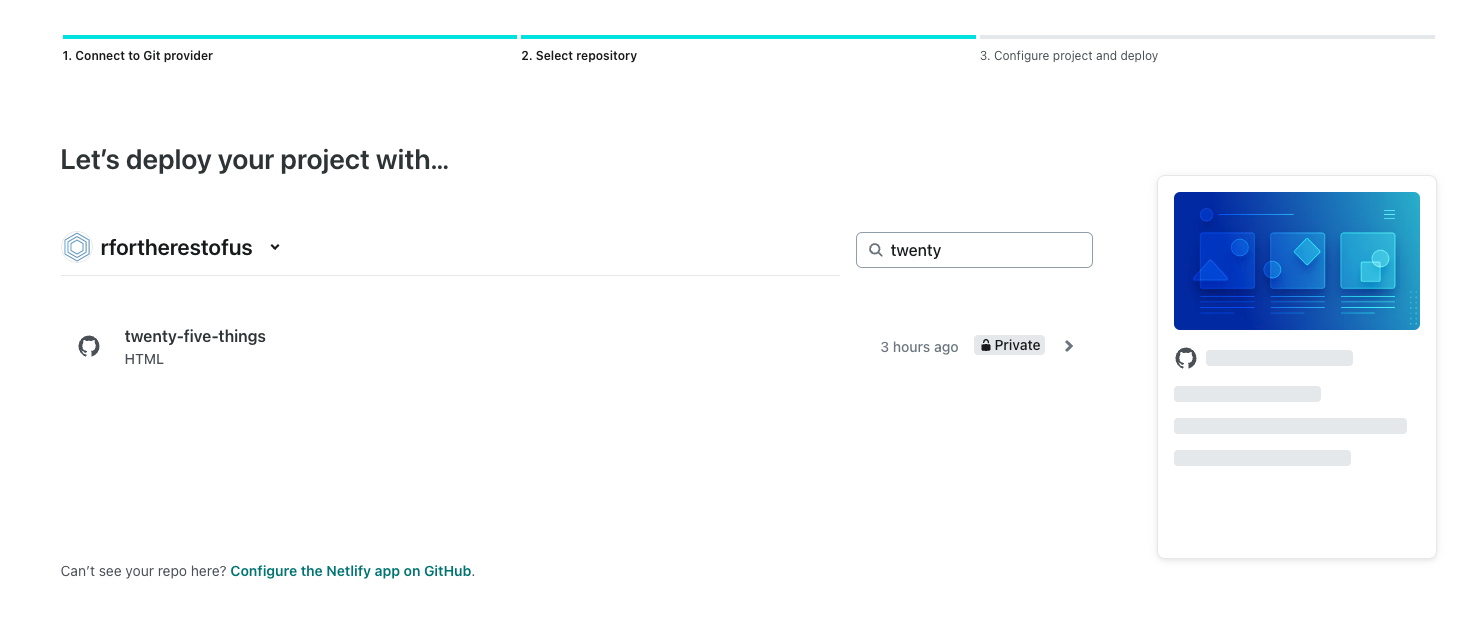
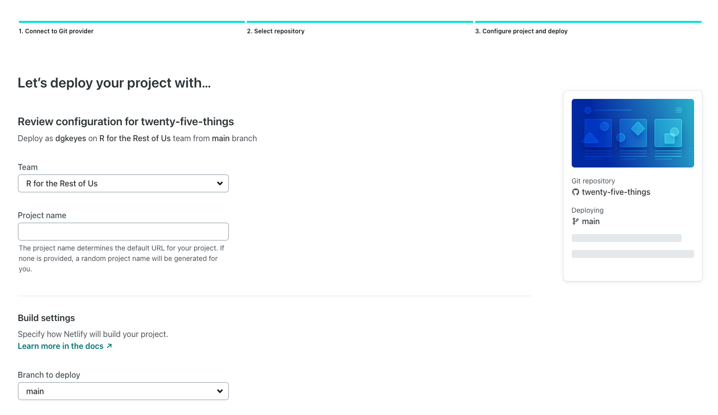
https://rfortherestofus.com/cascadia2025

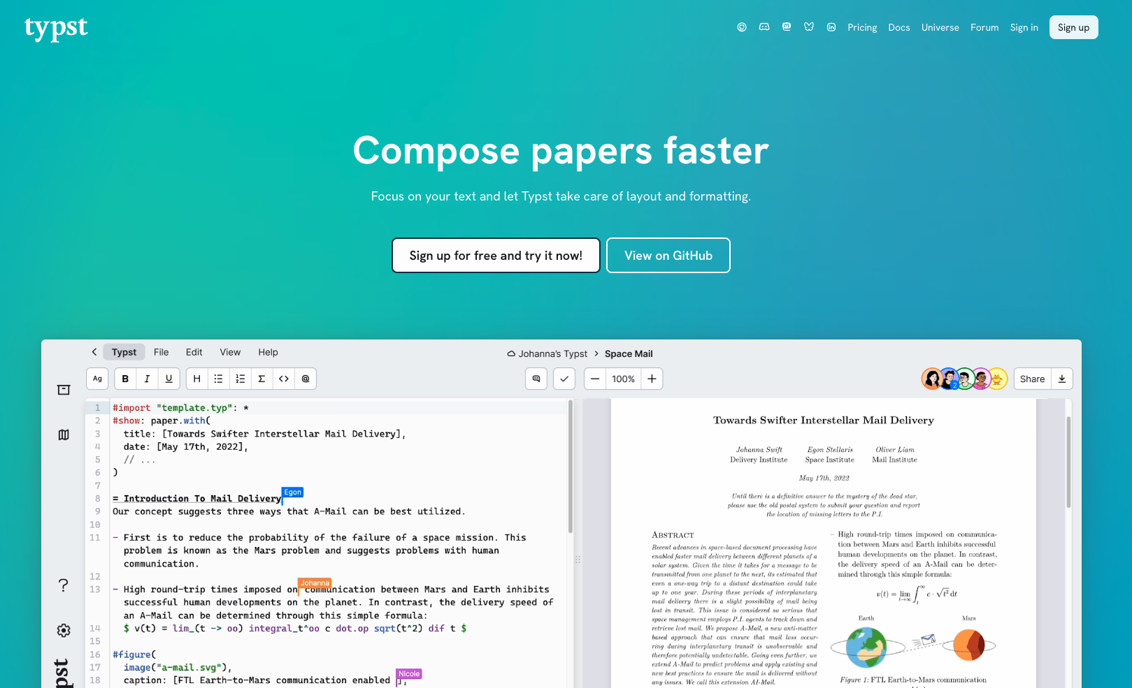
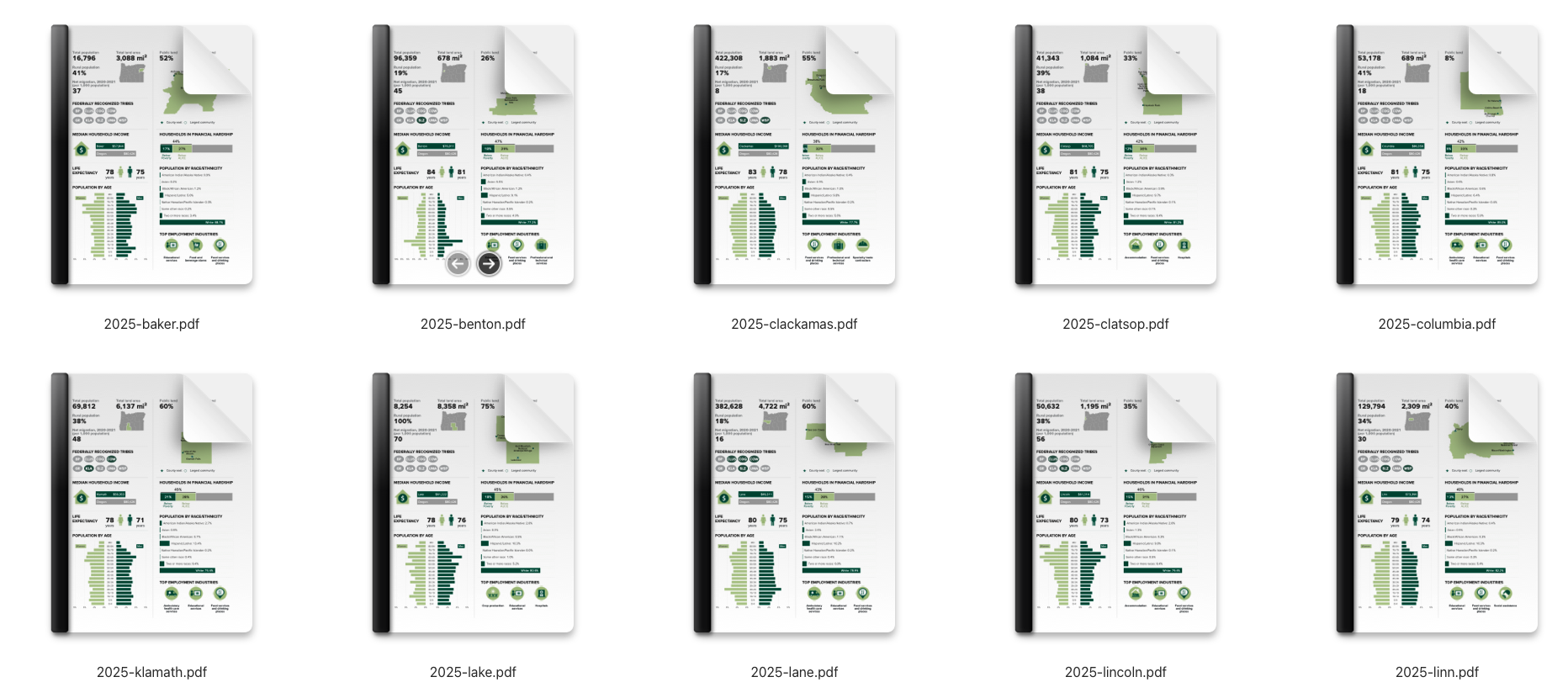
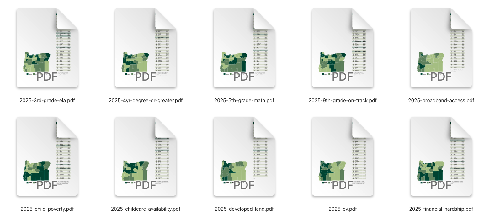
Make PDFs with Typst

15

Most people, when they think about making PDFs in Quarto, immediately think Latex. If this is enough to put you off from making PDFs in R, please know there is a new alternative. Known as typst, it is a modern reimagining of Latex.

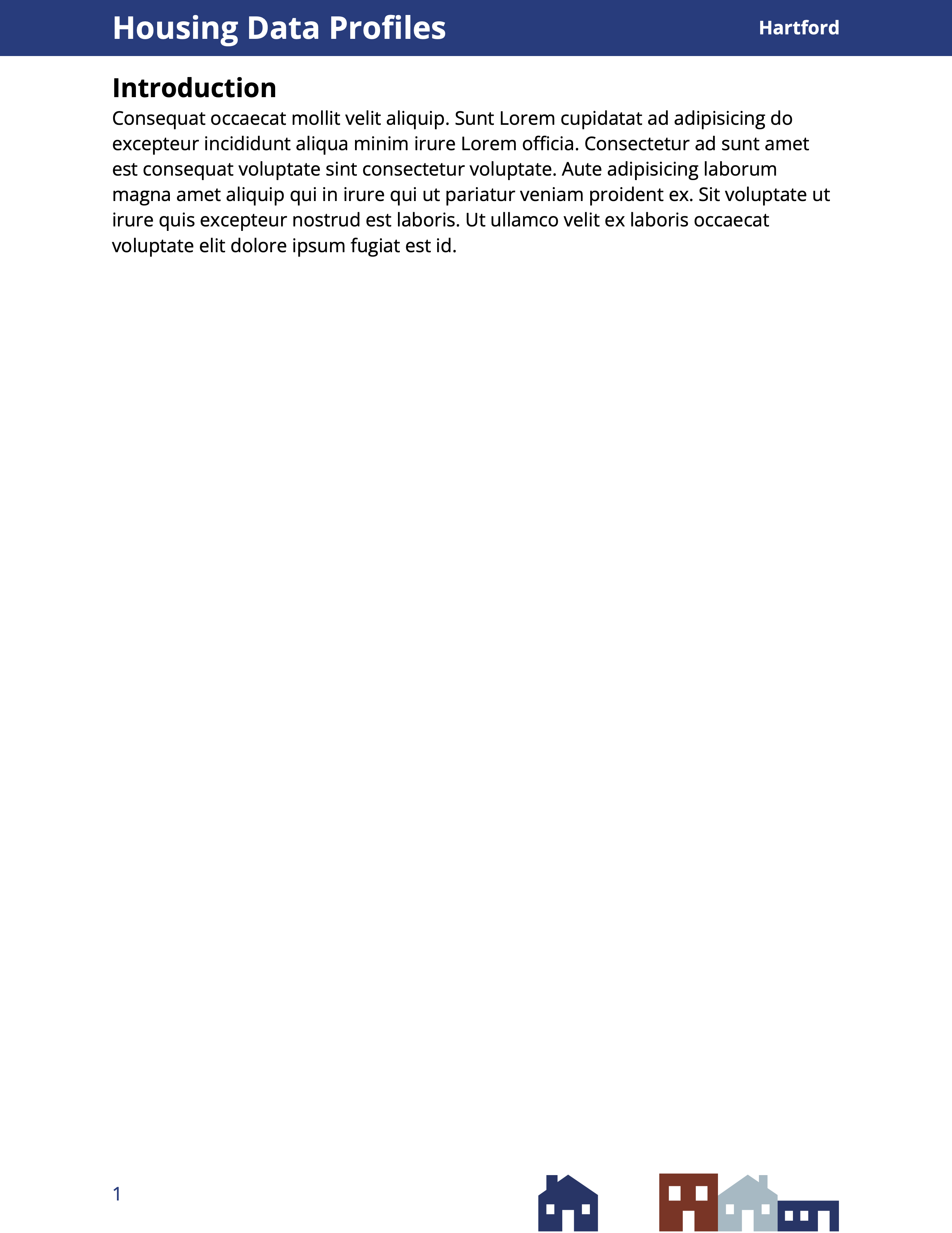
report.qmd

---
title: "Housing Data Profiles"

format: 
  typst:
    template-partials:
      - typst-show.typ
      - typst-template.typ

params:
  town: "Hartford"
---

# Introduction

Consequat occaecat mollit velit aliquip. etc ...

typst-show.typ

#show: psc-report.with(
  $if(title)$
    title: "$title$",
  $endif$
  $if(params.town)$
    town: "$params.town$",
  $endif$
)

typst-template.typ

#let psc-report(
  title: "title",
  town : "town",
  body,
) = {

 set text(
    font: "Open Sans",
    size: 12pt,
  )

 set page(
    "us-letter",
    margin: (left: 1in, 
             right: 1in, 
             top: 0.7in, 
             bottom: 1in),
    background: place(top, 
                      rect(fill: rgb("15397F"), 
                           width: 100%, 
                           height: 0.5in)),
    header: align(
      horizon,
      grid(
        columns: (80%, 20%),
        align(left, text(size: 20pt, fill: white, weight: "bold", title)),
        align(right, text(size: 12pt, fill: white, weight: "bold", town)),
      ),
    ),
    footer: align(
      grid(
        columns: (40%, 60%),
        align(horizon, text(fill: rgb("15397F"), 
                            size: 12pt, 
                            counter(page).display("1"))),
        align(right, image("assets/psclogo.svg", height: 300%)),
      )
    )
  )

  body
}

Automate all the Things

Email Your Reports Directly from R

16

In 2020, at the start of the COVID pandemic, we were working with Prosper Portland, the small business development agency for the city of Portland. They had quickly started a grant program for businesses impacted by the pandemic. It was, like so much in those early days of COVID, thrown together quickly. They set up an application form and they wanted an easy way to see a summary of information about businesses seeking relief. We wrote code to pull data from a Google Sheet and create a summary report. And, best of all, we set it up to email the report directly to Prosper Portland staff using the {gmailr} package.

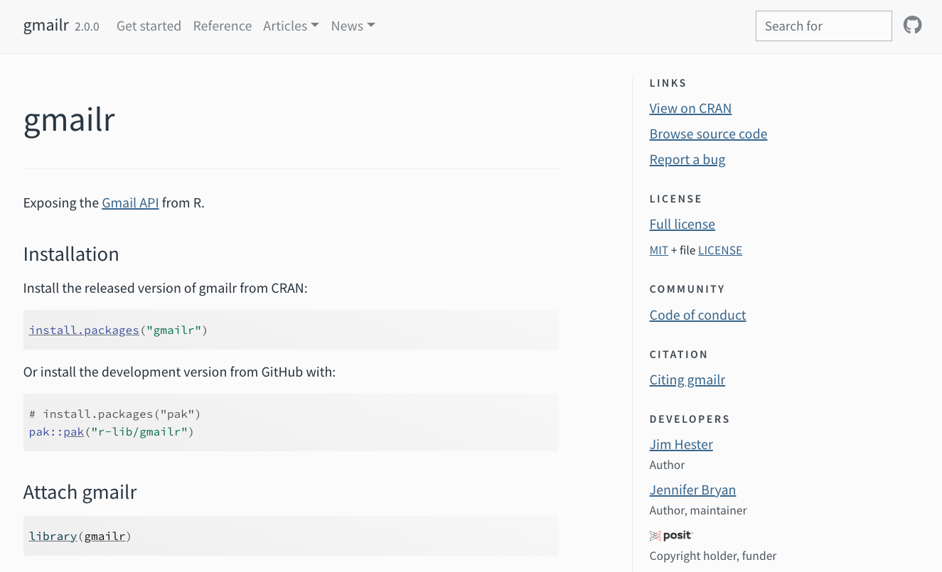
library(gmailr)

gm_auth_configure()
gm_auth(email = TRUE, cache = ".secret")

email_report <-
  gm_mime() |>
  gm_to("Joe Schmoe <joeschmoe@prosperportland.us>") |>
  gm_from("David Keyes <david@rfortherestofus.com>") |>
  gm_subject("COVID Business Relief Contact Log") |>
  gm_text_body("See attached") |>
  gm_attach_file("grant-report.html")

gm_send_message(email_report)

Run Your Code Without Lifting a Finger

17

When I talked about the daily reports we created for Prosper Portland, I left out one key thing: once we set up the code, we never ran it manually. How did we run the code to pull in the data, render the reports, and email them to Prosper Portland? With GitHub Actions. If you’ve never heard of GitHub Actions, it’s a tool that runs code on your behalf. You add a special YAML file to your GitHub repo and your code runs on a schedule. Magic!

send-report.yaml

name: Render Report and Send It

on:
  schedule:
    - cron:  '00 14 * * 1-5'

jobs:
  build:
    runs-on: ubuntu-latest
    
    env:
      GMAILR_APP: ${{ secrets.GMAILR_APP }}
      GMAILR_EMAIL: ${{ secrets.GMAILR_EMAIL }}

send-report.yaml (continued)

   steps:
      - name: Checkout Repository
        uses: actions/checkout@v2

      - name: Install dependencies
        run: |
          install.packages("remotes")
          remotes::install_cran("gmailr")
          ETC
        shell: Rscript {0}
          
      - name: Render + Send
        run: |-
          Rscript render_gmail.R

Use R to Work With Files Created in R

18

Speaking of automation, I often have to move files around. For example, when working on the annual Oregon by the Numbers Report, I make a ton of plots that I have to share with the graphic designer who lays out the report. I used to manually copy all of these files and upload them to Google Drive. But then I came across the {fs} and {zip} packages. I use {fs} to create a list of all the files I’ve created, which I then pass to the {zip} package in order to create a zip file. And, if I’m feeling extra fancy, I upload the zip file automatically to Google Drive using the {googledrive} package. With all of this, I just have to run my code and share a single link with the designer.

library(fs)
library(zip)

county_pages <- dir_ls("outputs/pages/county/")

measure_pages <- dir_ls("outputs/pages/measure/")

zip(
  zipfile = str_glue("outputs/zip/obtn-files.zip"),
  files = c(county_pages, measure_pages)
)

library(googledrive)

drive_upload("outputs/zip/obtn-files.zip")

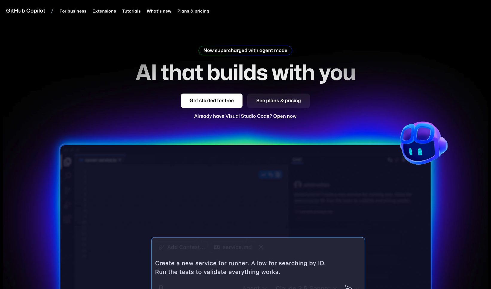
Use AI to Write Better Code

Let’s finish off by talking about ways that you can use large language models when working with R. Now I’m not an AI hype boy here to tell you that this or that model will blow your mind. And, to be honest, I’m actually a bit hesitant to discuss AI at all because what I tell you today may already be out of date. That said, I think there are some foundational ways that you can use LLMs that will stand the test of time.

Create Custom Instructions

19

My initial foray into using LLMs to work with code was, as I suspect was the case for many of you, through asking ChatGPT questions. And, like many of you, I found its answers at times incredibly helpful and at other times incredibly maddening. Sometimes it would give me base R code, other times tidyverse code. What I came to realize is that I needed to give it detailed instructions on what I wanted. And the best way to do this is to create custom instructions. Now, every time I ask an R question to an LLM, I do it with the following instructions:

Please answer the following R question. When I program, I always like to use the tidyverse. Please don’t ever give me base R solutions. Please also always use the native pipe (|>) not the tidyverse pipe (|>).

You can paste in instructions like this each time you work with your AI tool of choice. You can create custom GPTs in ChatGPT to save these custom instructions. I use a tool called Raycast for working with LLMs and it has a feature that allows me to create a custom AI prompt with these instructions.

Every time I have a question for AI, I call up my AI chat preset, which has my instructions embedded in it, and get out answers tailored to my desired style of coding.

Please answer the following R question.

When I program, I always like to use the tidyverse.

Please don’t ever give me base R solutions.

Use AI Directly in your Code Editor

20

Working with a tool like Raycast or ChatGPT requires you to go outside of your code editor. Another approach is to work with LLMs directly in your editor. If you use RStudio, you can connect directly with GitHub Copilot. If you use Positron, there are a number of extensions you can use to have LLMs interact directly with your code. Whether it’s offering suggestions on improving your code, adding new code, or asking general questions about your code, these tools can be extremely helpful.

Show AI Your Data

21

A few months ago, I spoke with Posit developer Simon Couch, who is working on a range of R packages to interact with LLMs. Simon has written that:

Data science differs a bit from software engineering here, though, in that the state of your R environment is just as important (or more so) than the contents of your files.

In our conversation, Simon explained this further, saying that, when asking a question to an LLM, it’s useful if it can see what the objects in your environment look like. The {gander} package solves this problem by passing information about your data frames alongside whatever request you make of an LLM.

Data science differs a bit from software engineering … in that the state of your R environment is just as important (or more so) than the contents of your files.

── system ──────────────────
You are a helpful but terse R data scientist. 
Respond only with valid R code: no exposition, no backticks. 
Always provide a minimal solution and refrain from unnecessary additions. 
Use tidyverse style and, when relevant, tidyverse packages. 
For example, when asked to plot something, use ggplot2, 
or when asked to transform data, using dplyr and/or tidyr unless 
explicitly instructed otherwise. 

── user ────────────────────
Up to this point, the contents of my r file reads: 
  
library(tidyverse)
library(sf)
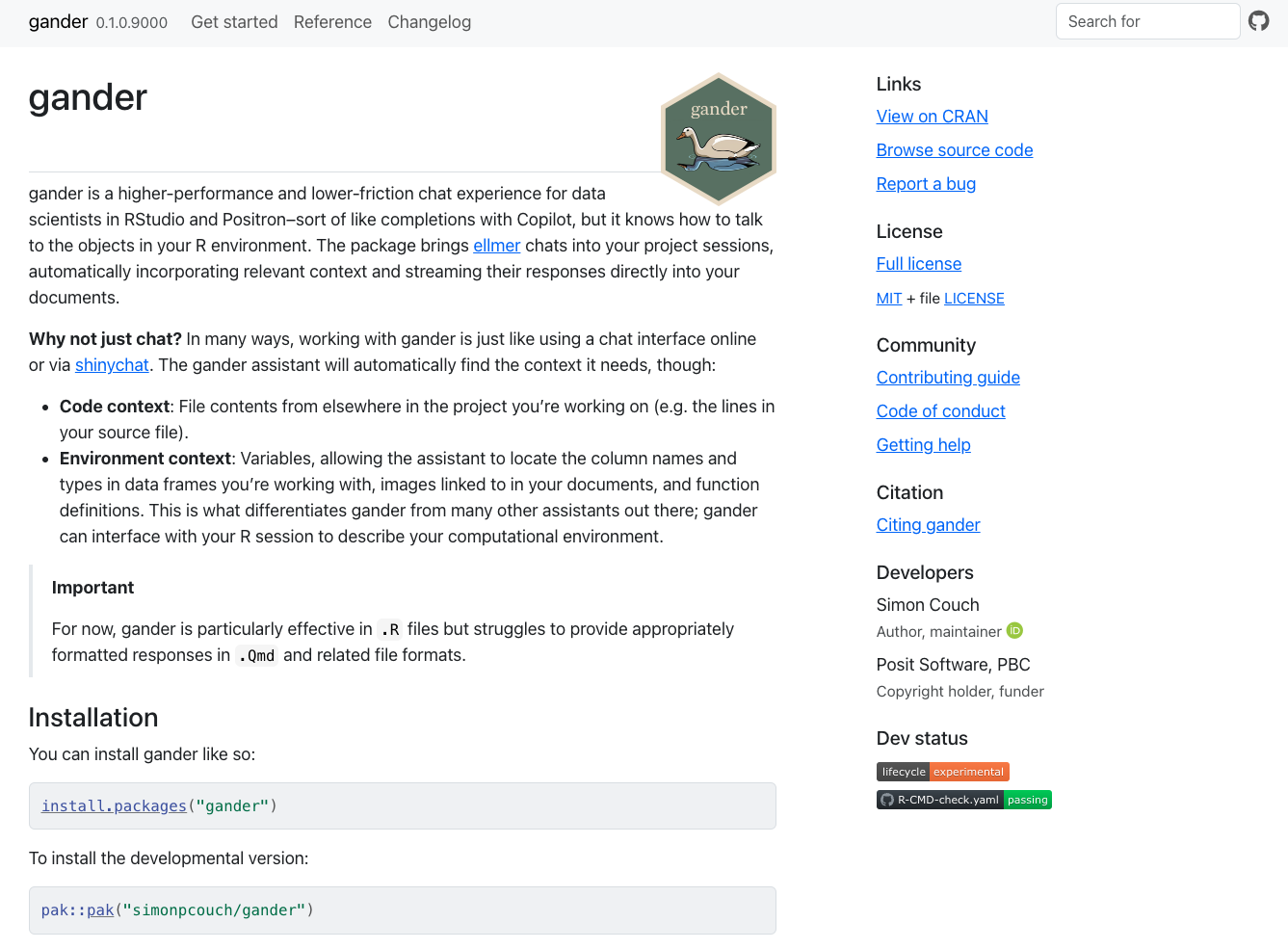
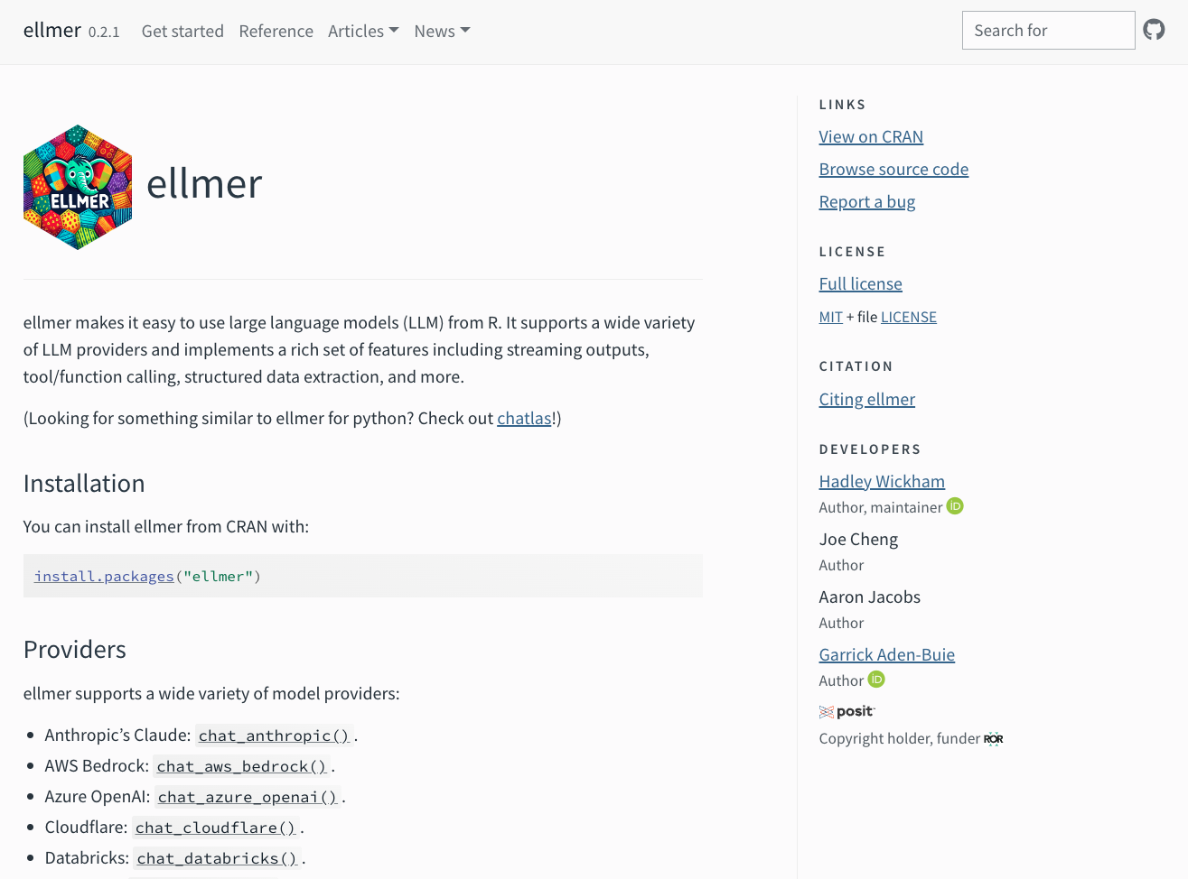
library(gander)

portland_boundaries <- read_sf("data/portland_boundaries.geojson")
pps_elementary_schools <- read_sf("data/pps_elementary_schools.geojson")

Now, Write code to tell me which schools are within Portland boundaries 

Here's some information about the objects in my R environment: 

```
# Just the first 1 row and 6 columns:
portland_boundaries
#> sf [1 × 6] (S3: sf/tbl_df/tbl/data.frame)
#>  $ objectid    : int 35
#>  $ cityname    : chr "Portland"
#>  $ shape_length: num 277321
#>  $ shape_area  : num 7.66e+08
#>  $ area        : num 4.05e+09
#>  $ geometry    :sfc_MULTIPOLYGON of length 1; first list element: List of 4
#>   ..$ :List of 13
#>   .. ..$ : num [1:14525, 1:2] -123 -123 -123 -123 -123 ...
#>   .. ..$ : num [1:642, 1:2] -123 -123 -123 -123 -123 ...
#>   .. ..$ : num [1:118, 1:2] -123 -123 -123 -123 -123 ...
#>   .. ..$ : num [1:5, 1:2] -122 -122 -122 -122 -122 ...
#>   .. ..$ : num [1:4, 1:2] -122.5 -122.5 -122.5 -122.5 45.5 ...
#>   .. ..$ : num [1:676, 1:2] -123 -123 -123 -123 -123 ...
#>   .. ..$ : num [1:11, 1:2] -122 -122 -122 -122 -122 ...
#>   .. ..$ : num [1:20, 1:2] -123 -123 -123 -123 -123 ...
#>   .. ..$ : num [1:4, 1:2] -122.7 -122.7 -122.7 -122.7 45.5 ...
#>   .. ..$ : num [1:10, 1:2] -122 -122 -122 -122 -122 ...
#>   .. ..$ : num [1:28, 1:2] -123 -123 -123 -123 -123 ...
#>   .. ..$ : num [1:57, 1:2] -123 -123 -123 -123 -123 ...
#>   .. ..$ : num [1:75, 1:2] -123 -123 -123 -123 -123 ...
#>   ..$ :List of 1
#>   .. ..$ : num [1:6, 1:2] -123 -123 -123 -123 -123 ...
#>   ..$ :List of 1
#>   .. ..$ : num [1:189, 1:2] -123 -123 -123 -123 -123 ...
#>   ..$ :List of 1
#>   .. ..$ : num [1:5, 1:2] -123 -123 -123 -123 -123 ...
#>   ..- attr(*, "class")= chr [1:3] "XY" "MULTIPOLYGON" "sfg"
#>  - attr(*, "sf_column")= chr "geometry"
#>  - attr(*, "agr")= Factor w/ 3 levels "constant","aggregate",..: NA NA NA NA NA
#>   ..- attr(*, "names")= chr [1:5] "objectid" "cityname" "shape_length" "shape_area" ...

# Just the first 5 rows and 2 columns:
pps_elementary_schools
#> sf [5 × 2] (S3: sf/tbl_df/tbl/data.frame)
#>  $ school  : chr [1:5] "Lenox Elementary School" "Cedar Mill Elementary School" "Montclair Elementary School" "Raleigh Hills Elementary School" ...
#>  $ geometry:sfc_POINT of length 5; first list element:  'XY' num [1:2] -122.9 45.6
#>  - attr(*, "sf_column")= chr "geometry"
#>  - attr(*, "agr")= Factor w/ 3 levels "constant","aggregate",..: NA
#>   ..- attr(*, "names")= chr "school"

Use AI for Data Analysis

LLMs are great for helping you write code to analyze your data. They can also do some of the data analysis for you.

Now, before anything else, I have to say: please don’t rely on LLMs for mission critical analysis without manually reviewing its work. Hallucinations are real.

With that said, the area I have found LLMs to be most helpful is with qualitative data. This data, which is often unstructured, is a perfect candidate for a tool that is comfortable bringing structure to messiness. Here are a few ways you can use it.

Translate Text

22

The {mall} package can also translate text. If you get responses in multiple languages, you can easily translate them to English.

library(tidyverse)

survey_spanish <-
  read_csv("data/survey_spanish.csv")

library(mall)

survey_translated <-
  survey_spanish |>
  llm_translate(spanish, language = "English", pred_name = "english")

Summarize Text

23

If you’ve ever conducted a survey or simply asked an open-ended question and got more text back than you could analyze by hand, why not try using AI for a quick and dirty analysis? The {mall} package lets you take long text and summarize it down to a shorter length.

References - https://mlverse.github.io/mall/#summarize

survey_translated_summary <-
  survey_translated |>
  llm_summarize(english, max_words = 5, pred_name = "summary")

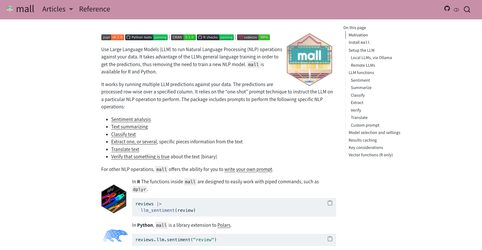
Create your Own Prompt to Analyze Text

24

The {mall} package provides some great out-of-the-box prompts you can use. You can also create your own prompts. I’ve used the {ellmer} package to interact directly with LLMs.

Here, for example, I created my own function using {ellmer} to identify themes from a set of survey responses.

library(ellmer)

identify_themes <- function(text) {
  chat <- chat_openai(
    system_prompt = "You are a sociologist,
    looking for the top three themes in the responses to a survey.
    Each response is separated by \n"
  )

  chat$chat(text)
}

survey_translated_combined <-
  survey_translated |>
  pull(english) |>
  paste(collapse = "\n")

[1] "Allows the handling of multiple statistical procedures that are difficult to perform in other programs.\nThe power and multitude of packages available for almost anything\nThe community of users (there's always an answer to every problem you find)\nThere are many development options available with good documentation.\nThe flexibility at the time of data management. In R, it's not what you can do with the data, but how.\nAllows me to process data of any type with sufficient accuracy, in addition to allowing exploration of creativity through report design using markdown.\nI like speed with which I can solve a problem and feel sure that I am doing it correctly, because many professional experts have invested time in the packages and solutions.\nThe ease of tidyverse, R Markdown, the diversity of packages, options, a large community of support, and data visualization tools.\nThe possibility of performing various tasks with a single software that is free and has a large and generous community of users sharing their knowledge."

survey_translated_combined |>
  identify_themes()

Based on the survey responses provided, the top three themes appear to be:

1. **Open Source and Community Contributions**: Many responses highlight the benefits of R being open-source, emphasizing the cost-free access to robust 
data analysis tools and frequent updates driven by community contributions. The active community also offers a wealth of packages for various tasks, which
enhances the flexibility and capability of the software.

2. **Learning and Accessibility**: While there is mention of a steep learning curve initially, respondents note that learning R becomes easier over time. The diversity and availability of resources make it possible to quickly achieve results, encouraging continued learning and exploration.


3. **Functionality and Efficiency**: Respondents appreciate the range of statistical procedures that R can handle with ease, as well as the speed and efficiency in managing large datasets. The power of R's data structure, which aligns with mathematical concepts, and the wide variety of packages further contribute to its functionality.

I’ve now given you 24 things that you perhaps didn’t know you could do with R. All of them are technical. But I’d be remiss if I didn’t mention the one thing that you can do with R that is, in fact, the opposite of technical.

When I started learning R, I never expected to find such a strong, welcoming community. But that’s exactly what I’ve found. R has technical power, sure. But it also has the ability to bring a wide range of people together on a beautiful Saturday to sit all day in an air conditioned room.

Join the Community

25

You may not have ever considered it, but R can help you find your community. As you learn from others today, I hope that you will consider giving back to maintain and improve the wonderful R community that we all gain so much from.

That I, a qualitative researcher who, for so long, thought of myself as not being a “real” user am up here today is in no small part because of the encouragement I have received from the R community. It may be a technical tool that brings us together in the first place, but it is the community that keeps us together in the long run.